empir_ARL2_profile.m
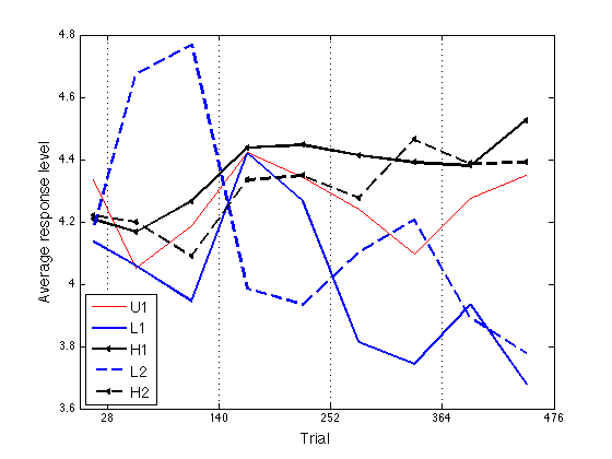
Final plot of the empirical Avg Response Levels w/ 56-trial blocks. See Figures 4 and 5 in ProtoPaper/expmt.tex. Compare with model_ARL2_predictions.m
File: work/CMUExper/fdbk1/data/empir_ARL2_profile.m
Date: 2007-08-12
Alexander Petrov, http://alexpetrov.com
Contents
- Load Fdbk1 human data
- Group descriptors
- Collapse across groups
- Group the points in pairs
- Save the ARL2 profiles for subsequent fits
- Plot the ARL profile. Same LineStyles as model_ARL2_predictions.
- Export ARL2 to SPSS in ASCII format
- Export same ARL2 to SSPS, rearranging for within-sbj ANOVA
- Define Assimilation := ARL(N)-ARL(P) and plot Assim profile
- Multiple Regression (ANCOVA) on the Assim group data
- Full model
- Model without interaction terms
- Significance of the Time covariate
- Significance of the Fdbk factor
- Significance of the Order factor
- Clean up
Load Fdbk1 human data
ARL is calculated as in the CatRat1 experiment
See work/CMUExper/CatRat1/data/trend/
clear all ;
cd(fullfile(work_pathstr,'CMUExper','fdbk1','data')) ;
load('S.mat') ;
idx = find([S(:).sbj_number]>=99) ;   % eliminate pilot runs
S(idx) = [] ;
ARL = [S(:).ARL] ;    % 17x55
Group descriptors
gr=[S(:).group]' ;
xtab1(gr)
fdbk_first_p = [1 1 1 0 0 0] ;    % exp schedule by group
%gr_descr = {'Ufb','Pfb','Nfb','xxx','Pno','Nno' } ;
gr_descr = {'U1','L1','H1','xxx','L2','H2' } ;
   Value   Count  Percent  Cum_cnt  Cum_pct
-------------------------------------------
       1      11    20.00       11    20.00
       2      11    20.00       22    40.00
       3      11    20.00       33    60.00
       5      11    20.00       44    80.00
       6      11    20.00       55   100.00
-------------------------------------------
Collapse across groups
grARL = zeros(size(ARL,1),max(gr)) ;   % 17x6
for k = 1:max(gr)
    idx = find(gr==k) ;
    if (~isempty(idx))
        grARL(:,k) = mean(ARL(:,idx),2) ;
    end
end
grARL
grARL =
    4.3358    4.1354    4.2075         0    4.1789    4.2197
    4.0411    4.0838    4.1610         0    4.4570    4.3693
    4.0639    4.0350    4.1723         0    4.8891    4.0287
    4.1521    4.0537    4.2286         0    4.8043    4.1585
    4.2236    3.8352    4.3046         0    4.7330    4.0194
    4.3239    4.3174    4.4587         0    4.0544    4.2597
    4.5233    4.5207    4.4153         0    3.9155    4.4074
    4.3777    4.2732    4.4184         0    4.0007    4.3081
    4.3067    4.2592    4.4738         0    3.8678    4.3894
    4.3178    3.8628    4.4319         0    3.9486    4.2385
    4.1629    3.7666    4.3952         0    4.2545    4.3144
    4.0674    3.7753    4.3084         0    4.1976    4.4453
    4.1249    3.7122    4.4734         0    4.2139    4.4834
    4.2917    3.9530    4.2607         0    3.9207    4.3365
    4.2568    3.9123    4.4973         0    3.8637    4.4364
    4.3501    3.6305    4.5398         0    3.8915    4.3348
    4.3486    3.7241    4.5097         0    3.6673    4.4448
Group the points in pairs
The difference between this and re-fitting the ARLs over 56-trial windows is less than 1%. I checked it on synthetic data. The problem is that data_by_sbj.m does it with 28-trial blocks and takes care of missing values. There is no need to redo this, given that the outcome will be virtually the same.
idx = [2:2:16]' ;
grARL2 = (grARL(idx,:)+grARL(idx+1,:))./2 ;
grARL2 = [grARL(1,:) ; grARL2]               % 9x6

ARL2 = (ARL(idx,:)+ARL(idx+1,:))./2 ;
ARL2 = [ARL(1,:) ; ARL2] ;                   % 9x55
grARL2 =
    4.3358    4.1354    4.2075         0    4.1789    4.2197
    4.0525    4.0594    4.1666         0    4.6730    4.1990
    4.1878    3.9444    4.2666         0    4.7687    4.0890
    4.4236    4.4190    4.4370         0    3.9850    4.3336
    4.3422    4.2662    4.4461         0    3.9343    4.3488
    4.2404    3.8147    4.4136         0    4.1016    4.2765
    4.0962    3.7438    4.3909         0    4.2058    4.4644
    4.2742    3.9327    4.3790         0    3.8922    4.3864
    4.3494    3.6773    4.5247         0    3.7794    4.3898
Save the ARL2 profiles for subsequent fits
S2 = S ;
for k = 1:length(S)
    S2(k).ARL2 = ARL2(:,k) ;
end
save S2 S2
Plot the ARL profile. Same LineStyles as model_ARL2_predictions.
ls = {'r-' 'b-' 'k<-' 'r--' 'b--' 'k<--'} ;   % group line styles
lw = [1 2 2  1 2 2] ;                         % group line widths
%lw = [.5 1.5 1.5  .5 1.5 1.5] ;               % group line widths

x2 = [14 , 56:56:448]' ;
xtick = [28 , 140:112:476] ;
ytick = [3.6:.2:4.8] ;
ax = [0 476 3.6 4.8] ;

clf ; hold on ;
for k = unique(gr)'
    hh = plot(x2,grARL2(:,k),ls{k}) ;
    set(hh,'LineWidth',lw(k),'MarkerSize',4) ;
end
hold off ; box on ;
axis(ax) ; set(gca,'xtick',xtick,'ytick',ytick,'xgrid','on') ;
hh = xlabel('Trial') ; set(hh,'FontSize',14) ;
hh = ylabel('Average response level') ; set(hh,'FontSize',14) ;
hh = legend('U1','L1','H1','L2','H2',3) ; set(hh,'FontSize',14) ;
% Saved as work/papers/ProtoPaper/fig/ARL-empir.pdf
Export ARL2 to SPSS in ASCII format
Write a text file with one row per data point and the following columns:
- 1. Sbj -- 1-55
- 2. Group -- 1=U1, 2=L1, 3=H1, 5=L2, 6=H2
- 3. Context -- 1=U, 2=L, 3=H
- 4. Order -- 1=Feedback_first, 2=No_feedback_first
- 5. Block -- 1-9. Each is 56 trials (except the first, which is 28).
- 6. Feedback -- 0=None, 1=Fdbk
- 7. ARL2
% Design matrix for each group
Context = [1 2 3 1 2 3] ;
Order = [1 1 1 2 2 2] ;
Feedback = [1 1 1 0 0 1 1 0 0 ;  ...    % when order=1
            1 0 0 1 1 0 0 1 1 ]' ;      % when order=2
Block = [1:9]' ;
Design = zeros([9 5 6]) ;     % 9 blocks x 5 variables x 6 groups
D = zeros(9,5) ;
for k = 1:6
    D(:,1) = k ;
    D(:,2) = Context(k) ;
    D(:,3) = Order(k) ;
    D(:,4) = Block ;
    D(:,5) = Feedback(:,Order(k)) ;
    Design(:,:,k) = D ;
end

% Data matrix with one row per point
data1 = zeros(0,7) ;
D = zeros(9,7) ;
for k = 1:length(S) ;
    D(:,1) = S(k).sbj_number ;
    D(:,2:6) = Design(:,:,S(k).group) ;
    D(:,7) = ARL2(:,k) ;
    data1 = [data1 ; D] ;
end

% Write to an ASCII file
fid = fopen('ARL2-bn-Ss.dat','w') ;
fprintf(fid,'Sbj Group Context Order Block Feedback ARL2\n') ;
for k = 1:size(data1,1)
    fprintf(fid,'%02d %1d %1d %1d %02d %1d %5.3f\n',data1(k,:)) ;
end
fclose(fid) ;
Export same ARL2 to SSPS, rearranging for within-sbj ANOVA
Write a text file with one row per subject and the following columns:
- 1. Sbj -- 1-55
- 2. Group -- 1=U1, 2=L1, 3=H1, 5=L2, 6=H2
- 3. Context -- 1=U, 2=L, 3=H
- 4. Order -- 1=Feedback_first, 2=No_feedback_first
- 5. W -- ARL2 value for the "warm-up" initial block
- 6-9. F1-F4 -- ARL2 values during the four feedback blocks
- 10-13. N1-N4 -- ARL2 values during the four no-feedback blocks
Note that this data format throws away the temporal order of observations. They are rearranged depending on Order so that in the resulting ASCII file all feedback ARLs are listed in columns F1-F4 and all no-feedback ARLs are listed in columns N1-N4.
Results of SPSS analyses available in work/CMUExper/fdbk1/data/SPSS/
rearrange = [1, 2 3 6 7, 4 5 8 9 ; ...     % when order=1
             1, 4 5 8 9, 2 3 6 7 ]' ;      % when order=2

data2 = zeros(length(S),13) ;
for k = 1:length(S)
    data2(k,1) = S(k).sbj_number ;
    hh = S(k).group ;
    data2(k,2:4) = Design(1,1:3,hh) ;
    data2(k,5:13) = ARL2(rearrange(:,Order(hh)),k)' ;
end

% Write to an ASCII file
fid = fopen('ARL2-wn-Ss.dat','w') ;
fprintf(fid,'Sbj Group Context Order W F1 F2 F3 F4 N1 N2 N3 N4\n') ;
for k = 1:size(data2,1)
    fprintf(fid,...
      '%02d %1d %1d %1d %5.3f %5.3f %5.3f %5.3f %5.3f %5.3f %5.3f %5.3f %5.3f\n',...
      data2(k,:)) ;
end
fclose(fid) ;
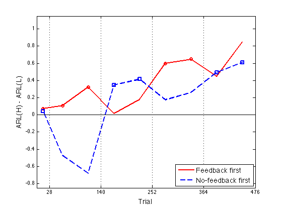
Define Assimilation := ARL(N)-ARL(P) and plot Assim profile
See CMUExper/fdbk1/data/assimil_profiles.m
- 1 = Feedback first = Group 3 - Group 2
- 2 = No-feedback first = Group 6 - Group 5
Assim = grARL2(:,[3 6]) - grARL2(:,[2 5])   % <-- Sic!

ax = [0 476 -0.85 1.15] ;
ytick1 = [-.8:.2:1] ;
idx1 = [1 2 3 6 7] ;    % feedback blocks for the feedback-first groups
idx2 = [1 4 5 8 9] ;    % feedback blocks for the no-feedback-first grps

clf ;
hh = plot(x2,Assim(:,1),'r-',x2,Assim(:,2),'b--',...
          x2(idx1),Assim(idx1,1),'ro',x2(idx2),Assim(idx2,2),'bs') ;
    set(hh,'LineWidth',2) ;
    axis(ax) ;
    hh=refline(0,0) ;
    set(hh,'Color','k','LineStyle','-','LineWidth',1) ;
box on ;
axis(ax) ; set(gca,'xtick',xtick,'ytick',ytick1,'xgrid','on') ;
hh = xlabel('Trial') ; set(hh,'FontSize',14) ;
hh = ylabel('ARL(H) - ARL(L)') ; set(hh,'FontSize',14) ;
hh = legend('Feedback first','No-feedback first',4) ; set(hh,'FontSize',14) ;
% Saved as work/papers/ProtoPaper/fig/Assim-empir.pdf
Assim =
    0.0720    0.0408
    0.1073   -0.4740
    0.3222   -0.6797
    0.0180    0.3486
    0.1799    0.4145
    0.5989    0.1749
    0.6471    0.2586
    0.4463    0.4943
    0.8474    0.6104
Multiple Regression (ANCOVA) on the Assim group data
Ignore the "warm-up" block 1. Regress the remaining 16 Assim points w.r.t the following predictors:
- 1. Time: 2-9
- 2. Feedback: -1=None, +1=Fdbk
- 3. Order: -1=No-fdbk-first, +1=Feedback-first
- 4. Fdbk X Order
Cf. David Howell (1992). "Statistical Methods for Psychology" (3rd Ed.). Chap. 16: ANOVA and ANCOVA as general linear models. Design matrix, p.553
y = reshape(Assim(2:9,:),16,1) ;    % dependent variable, N=16

X_Time = [2:9 , 2:9]' ;
X_Fdbk = [+1 +1 -1 -1 +1 +1 -1 -1 , -1 -1 +1 +1 -1 -1 +1 +1]' ;
X_Order = [ones(8,1) ; -ones(8,1)] ;
X_FxO = X_Fdbk .* X_Order ;

% Design matrix X
X = ones(16,1) ;                                   % Regression constant
X = [X (X_Time - mean(X_Time))./std(X_Time,1)] ;   % Standardize X_Time
X = [X X_Fdbk X_Order X_FxO]                       % Already standardized
X =
    1.0000   -1.5275    1.0000    1.0000    1.0000
    1.0000   -1.0911    1.0000    1.0000    1.0000
    1.0000   -0.6547   -1.0000    1.0000   -1.0000
    1.0000   -0.2182   -1.0000    1.0000   -1.0000
    1.0000    0.2182    1.0000    1.0000    1.0000
    1.0000    0.6547    1.0000    1.0000    1.0000
    1.0000    1.0911   -1.0000    1.0000   -1.0000
    1.0000    1.5275   -1.0000    1.0000   -1.0000
    1.0000   -1.5275   -1.0000   -1.0000    1.0000
    1.0000   -1.0911   -1.0000   -1.0000    1.0000
    1.0000   -0.6547    1.0000   -1.0000   -1.0000
    1.0000   -0.2182    1.0000   -1.0000   -1.0000
    1.0000    0.2182   -1.0000   -1.0000    1.0000
    1.0000    0.6547   -1.0000   -1.0000    1.0000
    1.0000    1.0911    1.0000   -1.0000   -1.0000
    1.0000    1.5275    1.0000   -1.0000   -1.0000
Full model
Use REGRESS in the STATS toolbox to do multiple regression. The regression coeff of Fx0 is not stat. diff. from 0:
[b_full,bint_full,r,rint,stats_full] = regress(y,X) ;
[b_full bint_full]'    % [Const Time Fdbk Order FxO]
stats_full             % [R2  F  p  MSE]
ans =
    0.2697    0.2738    0.1732    0.1262   -0.0308
    0.1778    0.1717    0.0814    0.0344   -0.1328
    0.3615    0.3759    0.2651    0.2180    0.0713
stats_full =
    0.8710   18.5597    0.0001    0.0278
Model without interaction terms
[b_main,bint_main,r,rint,stats_main] = regress(y,X(:,1:4)) ;
[b_main bint_main]'    % [Const Time Fdbk Order]
stats_main             % [R2  F  p  MSE]
rmse = sqrt(stats_main(4))
ans =
    0.2697    0.2872    0.1732    0.1262
    0.1809    0.1985    0.0845    0.0375
    0.3584    0.3760    0.2620    0.2150
stats_main =
    0.8658   25.8036    0.0000    0.0265
rmse =
    0.1629
Significance of the Time covariate
[b,bint,r,rint,stats] = regress(y,X(:,[1 3 4])) ;
R2_noTime = stats(1)
[F_Time,p] = R2signif(16,stats_main(1),3,R2_noTime,2)
R2_noTime =
    0.3097
Warning: Could not find an exact (case-sensitive) match for 'Fcdf'.
/Applications/MATLAB74/toolbox/stats/fcdf.m is a case-insensitive match and will be used instead.
You can improve the performance of your code by using exact
name matches and we therefore recommend that you update your
usage accordingly. Alternatively, you can disable this warning using
warning('off','MATLAB:dispatcher:InexactMatch').
F_Time =
   49.7215
p =
   1.3350e-05
Significance of the Fdbk factor
[b,bint,r,rint,stats] = regress(y,X(:,[1 2 4])) ;
R2_noFdbk = stats(1)
[F_Fdbk,p] = R2signif(16,stats_main(1),3,R2_noFdbk,2)
R2_noFdbk =
    0.6635
F_Fdbk =
   18.0880
p =
    0.0011
Significance of the Order factor
[b,bint,r,rint,stats] = regress(y,X(:,[1 2 3])) ;
R2_noOrder = stats(1)
[F_Order,p] = R2signif(16,stats_main(1),3,R2_noOrder,2)
R2_noOrder =
    0.7584
F_Order =
    9.6011
p =
    0.0092
Clean up
clear hh k idx D b bint r rint stats ;