fit_ANCHOR_ARL2_part1.m
Fit the ANCHOR2 model to the group ARL2 profiles of the Fdbk1 Experiment.
The main tool is .../work/models/anchor/fit_SSE/anchor_ARL2.m
File: work/CMUExper/fdbk1/data/fit_ANCHOR_ARL2_part1.m
Date: 2007-08-17
Alexander Petrov, http://alexpetrov.com
Contents
Load the data
clear all
cd(fullfile(work_pathstr,'CMUExper','fdbk1','data')) ;
load('S2.mat') ;
ARL2 = [S2(:).ARL2] ;    % 9x55
gr=[S2(:).group]' ;
ugr = unique(gr) ;
N_groups = length(ugr) ;
ugr_descr = {'U1' 'L1' 'H1', 'L2' 'H2' } ;   % [1 2 3, 5 6]
Collapse across groups
grARL2 = zeros(size(ARL2,1),N_groups) ;   % 9x5
gr_idx = cell(1,N_groups) ;
for k = 1:N_groups
    gr_idx{k} = find(gr==ugr(k))' ;
    grARL2(:,k) = mean(ARL2(:,gr_idx{k}),2) ;
end
grARL2
grARL2 =
    4.3358    4.1354    4.2075    4.1789    4.2197
    4.0525    4.0594    4.1666    4.6730    4.1990
    4.1878    3.9444    4.2666    4.7687    4.0890
    4.4236    4.4190    4.4370    3.9850    4.3336
    4.3422    4.2662    4.4461    3.9343    4.3488
    4.2404    3.8147    4.4136    4.1016    4.2765
    4.0962    3.7438    4.3909    4.2058    4.4644
    4.2742    3.9327    4.3790    3.8922    4.3864
    4.3494    3.6773    4.5247    3.7794    4.3898
Fit INST on the same stimulus sequences, 11 per group
stim = [S2(:).dist] ;   % 476x55
fdbk = [S2(:).fdbk] ;
Search parameters
Same as those used for fitting the INST model to the same profiles. See ./fit_INST_ARL2_part1.m for details
fminconp = 1 ;
flags = [0 1 1 0 0 0 0 0] ;   % [perc_k mem_k temper hist cutoff xx xx c_ratio]
Sparams = anchor_search_params2(flags,fminconp) ;
optns = optimset(Sparams.optns,'TolX',1e-2,'Display','off') ;
Sparams.optns = optns ;
Sparams.target_vals = grARL2
H = .040 ; Sparams.params.history = H ;   % for the time being
Sparams.params
Sparams =
     model_name: 'anchor_ARL2'
         params: [1x1 struct]
      p2v_templ: {'VAL = PARAMS.mem_k * 10 ;'  'VAL = PARAMS.temper * 10 ;'}
      v2p_templ: {'PARAMS.mem_k = VAL / 10 ;'  'PARAMS.temper = VAL / 10 ;'}
         bounds: [2x2 double]
     ARL_params: [1x1 struct]
    funfun_name: 'fmincon'
          optns: [1x1 struct]
     lsfun_name: 'sumsqerr'
    target_vals: [9x5 double]
ans =
       scale: 'LINEAR'
       N_cat: 7
     SM_conv: 1.0000e-03
      cat_sz: 0.0500
      perc_k: 0.0400
       mem_k: 0.0500
       avail: [7x1 double]
     anchors: [7x6 double]
     cutoffs: [-2.4000 -0.8000 0.5600 1.6800]
      temper: 0.0500
     history: 0.0400
       alpha: 0.3000
       decay: 0.5000
         ITI: 4
    M_raster: 7
    A_raster: [5 5 3 3]
    mnfieldp: 1
"Chance event" sets
The model is fitted using the deterministic version PROTOANCHOR_CHEV that uses previously cached values of all randomly generated values. More than one such "chev" sets is used to evaluate its impact on the fit.
N_chevs = 2 ;

% Pack into "model data" structures suitable for passing as arguments.
Mdata = cell(1,N_chevs) ;
for k = 1:N_chevs
    Mdata{k}.stim = stim ;
    Mdata{k}.fdbk = fdbk ;
    Mdata{k}.group_idx = gr_idx ;
    %Mdata{k}.params = Sparams.params ;    % will be set by SUMSQERR
    Mdata{k}.chev = make_anchor_chev(size(stim,1),size(stim,2),7) ;
    Mdata{k}.ARL_params = Sparams.ARL_params ;
end
Cutoff parameter grid
cutoff_levels = [.50 .55 .60 .65 .70 .75 .80 .85 .90]' ;  % c- in categ_sz units
N_cutoff_levels = length(cutoff_levels) ;
c_ratio_levels = [.5 .6 .65 .7 .75 .8 .9] ;         % c-/c+ ratio
N_c_ratio_levels = length(c_ratio_levels) ;
Main work
A grid search over 5x3x2 cells takes five hours on a fast machine. Therefore, the results will only be computed once and cached to disk.
fname = 'grid_search_ANCHOR_ARL2_part1.mat' ;
if (file_exists(fname))
    load(fname) ;
else
  grid_SSE = zeros([N_cutoff_levels,N_c_ratio_levels,N_chevs]) ;
  grid_optX = cell([N_cutoff_levels,N_c_ratio_levels,N_chevs]) ;
  grid_det = cell([N_cutoff_levels,N_c_ratio_levels,N_chevs]) ;
  tic
  for k1 = 1:N_cutoff_levels
      c = cutoff_levels(k1) ;
      fprintf('\n cutoff %4.2f: ',c) ;
      for k2 = 1:N_c_ratio_levels
          cr = c_ratio_levels(k2) ;
          cutoffs = c .* [-3 -1 cr 3*cr] ;
          Sparams.params.cutoffs = cutoffs ;
          for k = 1:N_chevs
              [par,SSE,optX,det] = paramsearch(Mdata{k},Sparams) ;  % <-- Sic!
              grid_SSE(k1,k2,k) = SSE ;
              grid_optX{k1,k2,k} = optX ;
              grid_det{k1,k2,k} = det ;
              fprintf('%5.3f ',SSE) ;
              save(fname,'grid_SSE','grid_optX','grid_det','Sparams',...
                   'cutoff_levels','c_ratio_levels') ;
          end
          fprintf(', ') ;
      end
  end
  fprintf('\n') ;
  toc
end % if file_exists ...
 cutoff 0.50: 2.872 3.045 , 2.182 1.684 , 1.213 1.490 , 1.051 1.683 , 1.023 1.049 , 1.230 1.120 , 1.749 1.442 ,
 cutoff 0.55: 2.928 2.990 , 2.134 1.640 , 1.122 1.648 , 1.632 1.138 , 1.007 1.059 , 1.227 1.044 , 1.867 1.356 ,
 cutoff 0.60: 2.915 2.575 , 1.325 1.610 , 1.070 1.644 , 1.092 1.152 , 1.033 1.013 , 1.245 1.108 , 1.892 1.483 ,
 cutoff 0.65: 2.563 2.948 , 1.986 1.958 , 1.630 1.255 , 1.014 1.159 , 1.032 1.019 , 1.366 1.143 , 1.936 1.593 ,
 cutoff 0.70: 2.560 2.533 , 1.900 1.442 , 1.526 1.306 , 1.027 1.163 , 1.162 1.069 , 1.363 1.181 , 1.894 1.777 ,
 cutoff 0.75: 2.408 2.447 , 1.876 1.769 , 1.081 1.215 , 0.982 1.135 , 1.229 1.099 , 1.361 1.272 , 2.155 1.655 ,
 cutoff 0.80: 2.390 2.523 , 1.628 1.433 , 1.069 1.250 , 1.044 1.155 , 1.188 1.118 , 1.390 1.262 , 2.081 1.910 ,
 cutoff 0.85: 2.317 2.329 , 1.283 1.517 , 1.031 1.178 , 1.058 1.117 , 1.266 1.087 , 1.446 1.361 , 2.074 1.916 ,
 cutoff 0.90: 2.527 2.351 , 1.483 1.462 , 1.187 1.159 , 1.153 1.124 , 1.245 1.208 , 1.495 1.356 , 2.295 2.044 ,
Elapsed time is 48095.056833 seconds.
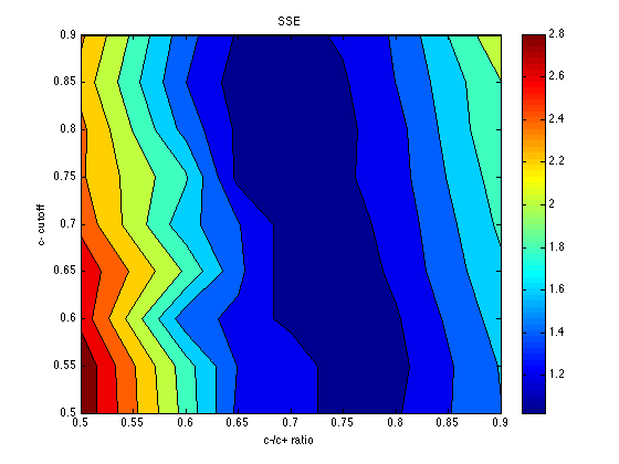
Plot the SSE
SSE = mean(grid_SSE,3)   % average across the chev's
[X,Y] = meshgrid(c_ratio_levels,cutoff_levels) ;
contourf(X,Y,SSE) ; colorbar ; title('SSE') ;
xlabel('c-/c+ ratio') ; ylabel('c- cutoff') ;
SSE =
    2.9584    1.9331    1.3514    1.3671    1.0363    1.1750    1.5956
    2.9592    1.8872    1.3848    1.3853    1.0330    1.1354    1.6115
    2.7446    1.4675    1.3571    1.1218    1.0230    1.1765    1.6877
    2.7557    1.9721    1.4425    1.0863    1.0251    1.2542    1.7649
    2.5465    1.6709    1.4160    1.0953    1.1153    1.2719    1.8356
    2.4274    1.8227    1.1479    1.0588    1.1638    1.3167    1.9050
    2.4567    1.5308    1.1599    1.0995    1.1530    1.3261    1.9958
    2.3231    1.4000    1.1041    1.0872    1.1768    1.4035    1.9949
    2.4389    1.4725    1.1729    1.1388    1.2267    1.4251    2.1695
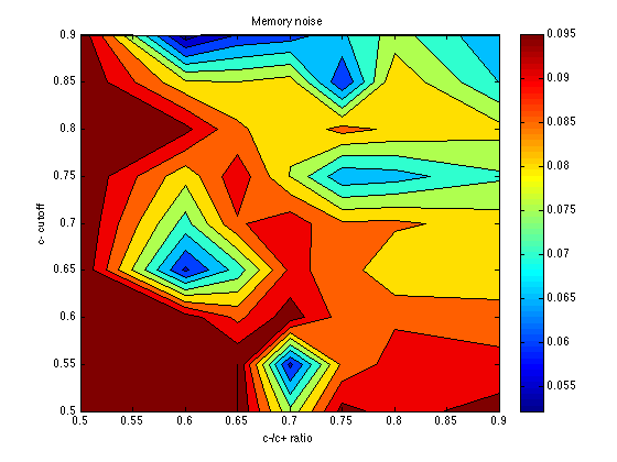
Plot the memory noise parameter
mem_k = zeros(size(grid_optX)) ;
temper = zeros(size(grid_optX)) ;
for k1 = 1:N_cutoff_levels
    for k2 = 1:N_c_ratio_levels
        for k = 1:N_chevs
            mem_k(k1,k2,k) = grid_optX{k1,k2,k}(1) / 10 ;
            temper(k1,k2,k) = grid_optX{k1,k2,k}(2) / 10 ;
        end
    end
end

mem_k = mean(mem_k,3)
contourf(X,Y,mem_k) ; colorbar ; title('Memory noise') ;
xlabel('c-/c+ ratio') ; ylabel('c- cutoff') ;
mem_k =
    0.0992    0.0998    0.1000    0.0766    0.0968    0.0931    0.0973
    0.1000    0.0998    0.1000    0.0586    0.0863    0.0920    0.0915
    0.1000    0.0981    0.0887    0.0979    0.0878    0.0893    0.0873
    0.1000    0.0591    0.0722    0.0910    0.0884    0.0800    0.0813
    0.0999    0.0729    0.0894    0.0932    0.0854    0.0861    0.0824
    0.1000    0.0816    0.0934    0.0798    0.0663    0.0678    0.0742
    0.1000    0.0965    0.0861    0.0808    0.0867    0.0841    0.0817
    0.1000    0.0809    0.0801    0.0826    0.0601    0.0842    0.0699
    0.0995    0.0522    0.0607    0.0625    0.0691    0.0773    0.0657
Plot the temperature parameter
temper = mean(temper,3)
contourf(X,Y,temper) ; colorbar ; title('Softmax temperature') ;
xlabel('c-/c+ ratio') ; ylabel('c- cutoff') ;
temper =
    0.0799    0.0508    0.0331    0.0404    0.0268    0.0329    0.0347
    0.0792    0.0518    0.0408    0.0350    0.0272    0.0292    0.0290
    0.0720    0.0372    0.0468    0.0321    0.0284    0.0364    0.0334
    0.0659    0.0586    0.0433    0.0350    0.0297    0.0317    0.0361
    0.0517    0.0435    0.0472    0.0357    0.0343    0.0348    0.0391
    0.0499    0.0671    0.0372    0.0348    0.0310    0.0321    0.0360
    0.0530    0.0505    0.0402    0.0378    0.0392    0.0401    0.0407
    0.0466    0.0429    0.0407    0.0359    0.0411    0.0422    0.0380
    0.0643    0.0468    0.0392    0.0388    0.0412    0.0420    0.0425

Interim conclusion
Fix c_ratio = .75 once and for all
Explore  cutoff in the range [.55 .60 .65 .70]
Explore  history in the range  [.20 .30 .40 .50 .60]
Initial search value for mem_k = .085
Initial search value for temper = .030
The fitting effort continues in fit_ANCHOR_ARL2_part2.m
Clean up
clear k k1 k2 X Y ;